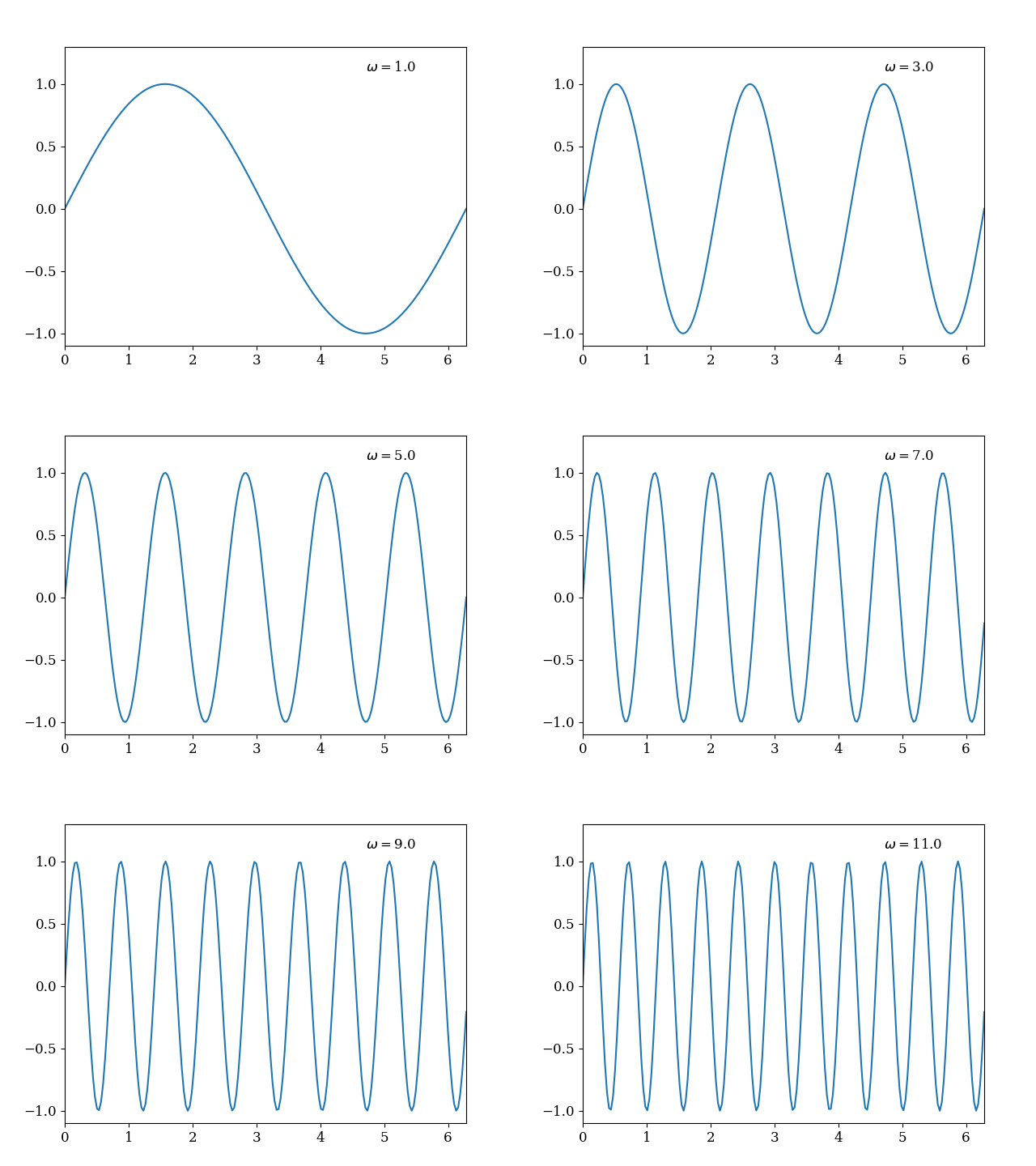
Sometimes the outcomes of our models are very complicated and are worth showing as a short video or animation. The best format for a short animation is a gif file. If the outcome is longer and contains more than ~100 frames it is better to use video format because they allow some additional compression.
In the following example I demonstrate how to create a simple animation using Python. One of the best discussions is available here. For the input function I will use the sinus with constantly increasing frequency.

First we import all packages which we use:
from pygifsicle import optimize
import os
import imageio
from math import *
import numpy as np
import matplotlib as mpl
import matplotlib.pyplot as plt
plt.rc('font', family='serif') ## setting for figures which I usually use in my publications
mpl.rcParams.update({'font.size': 12})
mpl.rcParams.update({'legend.labelspacing':0.25, 'legend.fontsize': 12})
mpl.rcParams.update({'errorbar.capsize': 4})
I change standard parameters for font in Matplotlib, so the final product can be inserted in an article. I use package pygifsicle to make the final gif more compact. In this example the file is compressed from 19 MB to 4.9 MB with a single command. Next I write a function which generates data for individual frame. Instead of data generation it is possible to read individual files in this function.
## Define a function which produces numerical input for our individual frame.
## It could be simply a fuction which reads individual files

def fun (i, x): ## argument of the function is the frame number

        return np.sin ((i/30.0+1)*x) ## we increase frequency in each frame
At the next stage we plot our data and save them as individual png files.
filenames = []

N = 300 ## Total number of separate frames in animation

x = np.linspace (0, 2*pi, 200)

for i in range (0, N):

        y = fun (i, x)

        plt.plot (x,y) #, rasterized=True)

        filename = 'frame_'+str(i)+'.png'

        filenames.append (filename)

        plt.xlim([0, 2.0*pi]) ## This adds stability to the axis
        plt.ylim([-1.1, 1.3])

        plt.text (1.5*pi, 1.1, r'$\omega=$'+str(round(i/30.0+1, 1)))

        plt.savefig (filename)
        #plt.show() ## this part could be used for debugging to see how individual frame looks like.
        plt.close()
plt.close() is used here to clean information from current plot, so the next frame does not have data shown at the previous frame. If our data are three-dimensional we can use plt.imshow() instead of plt.plot().
At the final step we call function get_writer from package imageio. This function combines all our individual figures into a single .gif file. After this step we can remove individual .png files.
gif_filename = 'sinus_gif.gif'

with imageio.get_writer(gif_filename, mode='I') as writer:
        for filename in filenames:  ## here we go through all prepared files
                image = imageio.imread(filename)
                writer.append_data(image)

                os.remove(filename) ## now we remove individual frames

optimize(gif_filename) ## to optimise the file size