Quite often it happens in science that the probability distribution is set only numerically at some grid. In this case, the fastest option is to prepare the numerical cumulative distribution by summing each element of the array. The cumulative distribution is inverted by means of a spline fitting procedure where the arguments are rearranged. The x-axis becomes the cumulative probability and y-axis is the actual random variable. After these steps, a sample with a uniform distribution between zero and one is easily converted by means of the fitted function to a distribution with the required probability density.
Here is an example in Python:
from scipy import interpolate
import numpy as np
from math import *
import matplotlib as mpl
import matplotlib.pyplot as plt
plt.rc('font', family='serif')
mpl.rcParams.update({'font.size': 12})
mpl.rcParams.update({'legend.labelspacing':0.25, 'legend.fontsize': 12})
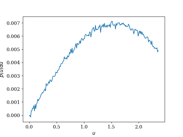
t = np.linspace(0, pi/2.0*1.5, 200) ## domain for numerical PDF is defined (grid)
rand_val = np.random.normal(0, 0.1, size=200)
y_diff = 5.3*np.sin (t) + rand_val
y_diff = y_diff / np.sum(y_diff) ## Actual numerical PDF
plt.plot(t, y_diff)
plt.xlabel(r'$u$')
plt.ylabel(r'$p(u)du$')
plt.savefig('pdf.png')
plt.show()
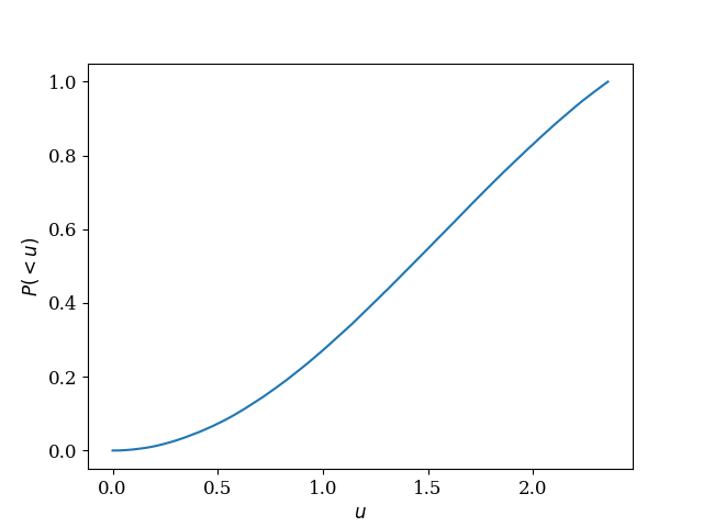
y_cumul = np.cumsum(y_diff, axis=0)
y_cumul = y_cumul / np.max(y_cumul) ## Preparing numerical cumulative distribution
plt.plot (t, y_cumul)
plt.xlabel(r'$u$')
plt.ylabel(r'$P(<u)$')
plt.savefig('cdf.png')
plt.show()
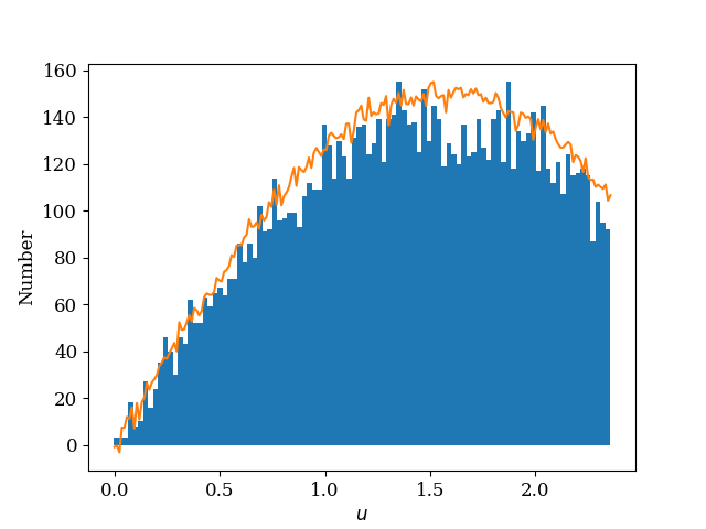
f = interpolate.interp1d(y_cumul, t, kind='cubic') ## fit the inverse (exchanged arguments) cumulative
y=np.random.uniform(np.min(y_cumul), np.max(y_cumul), size=10000) ## generate uniform distribution
sample = f(y) ## transform the uniform distribution to a distribution with required PDF using the
## spline interpolation
n, bins, patches = plt.hist(sample, bins=100)
plt.plot(t, y_diff / np.max(y_diff) * np.max(n))
plt.xlabel(r'$u$')
plt.ylabel('Number')
plt.savefig('result.png')
plt.show()
This is the actual numerical PDF: The cumulative distribution function: Here I draw a sample using the technique and compare it with the numerical PDF: